Graph Data Science with Neo4j

Full stack developer Meet/Discuss with me : https://cal.com/biomathcode
In GDS we refer to this process as projecting a graph and refer to the in-memory graph as a graph projection. GDS can hold multiple graph projections at once and they are managed by a component called the Graph Catalog.
This includes classic graph algorithms such as centrality, community detection, path finding, etc. It also includes embeddings, a form of robust graph feature engineering, as well as machine learning pipelines. There are a few things you may want to do with the output/result of graph algorithms. GDS enables you to write results back to the database, export to disk in csv format, or stream results into another application or downstream workflow.
In summary, read and load, execute and store
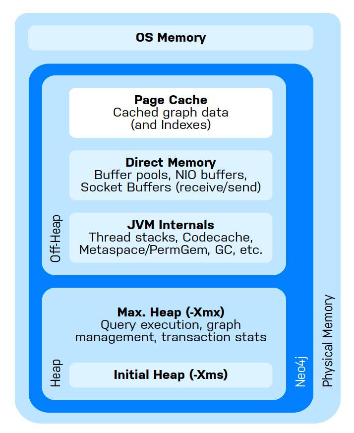
Of the above, two main types of memory can be allocated in configuration:
Heap Space: Used for storing in-memory graphs, executing GDS algorithms, query execution, and transaction state
Page Cache: Used for indexes and to cache the Neo4j data stored on disk. Improves performance for querying the database and projecting graphs.
Allocation of heap memory can be done with the dbms.memory.heap.initial_size and dbms.memory.heap.max_size in the Neo4j configuration
setting a minimum page cache size is still important when projecting graphs. This minimum can be estimated at approximately 8KB * 100 * readConcurrency for standard, native, projections. Page cache size can be set via dbms.memory.pagecache.size in the Neo4j configuration.
What is Graph Catalog?
creating (a.k.a projecting) graphs
viewing details about graphs
dropping graph projections
exporting graph projections
writing graph projection properties back to the database
How to work with GDS?
We create graph projection to create sparsh, so that we can run algorithms on them.
Then We can store the data from the algos, into node properties.
CALL gds.graph.nodeProperty.stream('my-graph-projection','numberOfMoviesActedIn')
YIELD nodeId, propertyValue
RETURN gds.util.asNode(nodeId).name AS actorName, propertyValue AS numberOfMoviesActedIn
ORDER BY numberOfMoviesActedIn DESCENDING, actorName LIMIT 10
For, example we can count the num of movie actor has acted in with data centrality algorithm.
We can also export data from the graphs,
two methods for that:
gds.graph.exportgds.beta.graph.export.csv
Dropping and deleting
CALL gds.graph.drop('my-graph-projection')
We list graphs
CALL gds.graph.list()
Native Projections
Native Projections provide the best performance and we can call gds.graph.project()
Syntax:
‘Name’, ‘Node project’, ‘relationshipProjection’
CALL gds.graph.project('native-proj',['User', 'Movie'], ['RATED']);
We set and use nodeProperites to Node and Relationship properties, as they can be used as weights in graph algo and features in ML.
CALL gds.graph.project(
    'native-proj',
    ['User', 'Movie'],
    {RATED: {orientation: 'UNDIRECTED'}},
    {
        nodeProperties:{
            revenue: {defaultValue: 0}, // (1)
            budget: {defaultValue: 0},
            runtime: {defaultValue: 0}
        },
        relationshipProperties: ['rating'] // (2)
    }
);
Why native projection are good ?
CALL gds.graph.project(
  'user-proj',
  ['User'],
  {
    SENT_MONEY_TO: { aggregation: 'SINGLE' }
  }
);
Sum Aggregator
CALL gds.graph.project(
  'user-proj',
  ['User'],
  {
    SENT_MONEY_TO: {
      properties: {
        totalAmount: {
          property: 'amount',
          aggregation: 'SUM'
        }
      }
    }
  }
);
Cypher Projections
Cypher projections are intended to be used in exploratory analysis and developmental phases where additional flexibility and/or customization is needed.
Syntax
A Cypher projection takes three mandatory arguments: graphName, nodeQuery, and relationshipQuery. In addition, the optional configuration parameter allows us to further configure graph creation.
Since we cannot do complex filtering in native project that is one of the reasons to use Cypher
CALL gds.graph.project.cypher(
  'proj-cypher',
  'MATCH (a:Actor) RETURN id(a) AS id, labels(a) AS labels',
  'MATCH (a1:Actor)-[:ACTED_IN]->(m:Movie)<-[:ACTED_IN]-(a2)
   WHERE m.year >= 1990 AND m.revenue >= 1000000
   RETURN id(a1) AS source , id(a2) AS target, count(*) AS actedWithCount, "ACTED_WITH" AS type'
);
Storing
CALL gds.degree.stream('proj-cypher',{relationshipWeightProperty: 'actedWithCount'})
YIELD nodeId, score
RETURN gds.util.asNode(nodeId).name AS name, score
ORDER BY score DESC LIMIT 10
Migrating from Cypher to native projection
//set a node label based on recent release and revenue conditions
MATCH (m:Movie)
WHERE m.year >= 1990 AND m.revenue >= 1000000
SET m:RecentBigMovie;

//native projection with reverse relationships
CALL gds.graph.project('proj-native',
  ['Actor','RecentBigMovie'],
  {
      ACTED_IN:{type:'ACTED_IN'},
    HAS_ACTOR:{type:'ACTED_IN', orientation: 'REVERSE'}
  }
);

//collapse path utility for relationship aggregation - no weight property
CALL gds.beta.collapsePath.mutate('proj-native',{
    pathTemplates: [['ACTED_IN', 'HAS_ACTOR']],
    allowSelfLoops: false,
    mutateRelationshipType: 'ACTED_WITH'
});
CALL gds.graph.project.cypher(
  // Projection name
  'movie-ratings-after-2014',
  // Cypher statement to find all nodes in projection
  'MATCH (m:Movie) RETURN id(m) AS id, labels(m) AS labels',
  // Cypher statement to find every User that rated a Movie
  // where the rating property is greater than or equal to 4
  // and the movie was released after 2014 (year > 2014)
  'MATCH (u:User)-[r:RATED]->(m:Movie)
   WHERE m.releaseYear > 2014 AND r.stars >= 4
   RETURN id(u) AS source , id(m) AS target, count(*) AS actedWithCount, "RATED" AS type'
) YIELD relationshipCount;
Solution
CALL gds.graph.project.cypher(
  // Projection name
  'movie-ratings-after-2014',
  // Cypher statement to find all nodes in projection
  '
    MATCH (u:User) RETURN id(u) AS id, labels(u) AS labels
    UNION MATCH (m:Movie) WHERE m.year > 2014 RETURN id(m) AS id, labels(m) AS labels
  ',
  // Cypher statement to find every User that rated a Movie
  // where the rating property is greater than or equal to 4
  // and the movie was released after 2014 (year > 2014)
  '
    MATCH (u:User)-[r:RATED]->(m:Movie)
    WHERE r.rating >= 4 AND m.year > 2014
    RETURN id(u) AS source,
        id(m) AS target,
        r.rating AS rating,
        "RATED" AS type
  '
);
Centrality and Importance
Centrality algorithms are used to determine the importance of distinct nodes in a graph.
Degree Centrality Example
IN GDS, we calcualte the no of out relationshhips from a node
Count the number of movies Actor has acted in
CALL gds.graph.project('proj', ['Actor','Movie'], 'ACTED_IN');
//get top 5 most prolific actors (those in the most movies)
//using degree centrality which counts number of `ACTED_IN` relationships
CALL gds.degree.stream('proj')
YIELD nodeId, score
RETURN gds.util.asNode(nodeId).name AS actorName, score AS numberOfMoviesActedIn
ORDER BY numberOfMoviesActedIn DESCENDING, actorName LIMIT 5
PageRank
PageRank estimates the importance of a node by counting the number of incoming relationships from neighboring nodes weighted by the importance and out-degree centrality of those neighbors. The underlying assumption is that more important nodes are likely to have proportionately more incoming relationships from other important nodes
//drop last graph projection
CALL gds.graph.drop('proj', false);

//create Cypher projection for network of people directing actors
//filter to recent high grossing movies
CALL gds.graph.project.cypher(
  'proj',
  'MATCH (a:Person) RETURN id(a) AS id, labels(a) AS labels',
  'MATCH (a1:Person)-[:DIRECTED]->(m:Movie)<-[:ACTED_IN]-(a2)
   WHERE m.year >= 1990 AND m.revenue >= 10000000
   RETURN id(a1) AS source , id(a2) AS target, count(*) AS actedWithCount,
    "DIRECTED_ACTOR" AS type'
);
Next stream PageRank to find the top 5 most influential people in director-actor network.
CALL gds.pageRank.stream('proj')
YIELD nodeId, score
RETURN gds.util.asNode(nodeId).name AS personName, score AS influence
ORDER BY influence DESCENDING, personName LIMIT 5
Betweenness Centrality: Measures the extent to which a node stands between the other nodes in a graph. It is often used to find nodes that serve as a bridge from one part of a graph to another.
Eigenvector Centrality: Measures the transitive influence of nodes. Similar to PageRank, but works only on the largest eigenvector of the adjacency matrix so does not converge in the same way and tends to more strongly favor high degree nodes. It can be more appropriate in certain use cases, particularly those with undirected relationships.
Article Rank: A variant of PageRank which assumes that relationships originating from low-degree nodes have a higher influence than relationships from high-degree nodes.
Path Finding
shortest path between two or more nodes and evaluate the availability and quality of path
Use Case, Supply chain analytics and Customer Journey
A Shortest Path:* An extension of Dijkstra that uses a heuristic function to speed up computation.
Yen’s Algorithm Shortest Path: An extension of Dijkstra that allows you to find multiple, the top k, shortest paths. [For multiple paths as well]
Dijkstra Single-Source Shortest Path: Dijkstra implementation for shortest path between one source and multiple targets.
Delta-Stepping Single-Source Shortest Path: Parallelized shortest path computation. Computes faster than Dijkstra single-source shortest Path but uses more memory.
CALL gds.graph.project('proj',
    ['Person','Movie'],
    {
        ACTED_IN:{orientation:'UNDIRECTED'},
        DIRECTED:{orientation:'UNDIRECTED'}
    }
);
MATCH (a:Actor)
WHERE a.name IN ['Kevin Bacon', 'Denzel Washington']
WITH collect(id(a)) AS nodeIds
CALL gds.shortestPath.dijkstra.stream('proj', {sourceNode:nodeIds[0], TargetNode:nodeIds[1]})
YIELD sourceNode, targetNode, path
RETURN gds.util.asNode(sourceNode).name AS sourceNodeName,
    gds.util.asNode(targetNode).name AS targetNodeName,
    nodes(path) as path;
Community Detection
group of nodes for clustering or Partitioned in the graph.
Louvain Community Detection
Louvain maximizes a modularity score for each community, where the modularity quantifies the quality of an assignment of nodes to communities. This means evaluating how much more densely connected the nodes within a community are, compared to how connected they would be in a random network.
hierarchical clustering
recursively merges communities together
stochastic algorithm
Label Propagation: Similar intent as Louvain. Fast algorithm that parallelizes well. Great for large graphs.
Weakly Connected Components (WCC): Partitions the graph into sets of connected nodes such that
- Every node is reachable from any other node in the same set 2. No path exists between nodes from different sets
Triangle Count: Counts the number of triangles for each node. Can be used to detect the cohesiveness of communities and stability of the graph.
Local Clustering Coefficient: Computes the local clustering coefficient for each node in the graph which is an indicator for how the node clusters with its neighbors
Code:
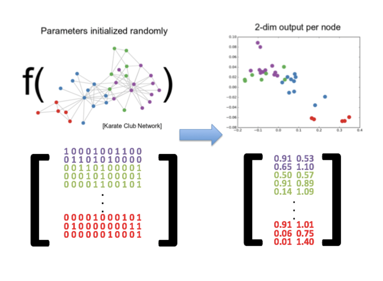
Node Embedding
node embedding is to compute low-dimensional vector representations of nodes such that similarity between vectors (eg. dot product) approximates similarity between nodes in the original graph.
Use Cases:
features for ML
Similarity Measurements
Exploratory Data Analysis(EDA)
FastRP
GDS offers a custom implementation of a node embedding technique called Fast Random Projection, or FastRP for short.
embeddingDimension: Applies to all node embedding algorithms in GDS. Controls the length of the embedding vectors. Setting this parameter is a trade-off between dimensionality reduction and accuracy.
IterationWeights: his controls two aspects: the number of iterations for intermediate embeddings, and their relative impact on the final node embedding. The parameter is a list of numbers, indicating one iteration per number where the number is the weight applied to that iteration
Example of FastRP
CALL gds.graph.project('proj', ['Movie', 'Person'], {
    ACTED_IN:{orientation:'UNDIRECTED'},
    DIRECTED:{orientation:'UNDIRECTED'}
});
Then Run FastRP
CALL gds.fastRP.stream('proj',  {embeddingDimension:64, randomSeed:7474})
YIELD nodeId, embedding
WITH gds.util.asNode(nodeId) AS n, embedding
WHERE n:Person
RETURN id(n), n.name, embedding LIMIT 10
Other Algo:
Node2Vec
GraphSage
Similarity
Similarity algorithms, as the name implies, are used to infer similarity between pairs of nodes
USe Cases:
Fraud Detection
Recommendation System
Entity Resolution
Algos:
Node Similarity: Determines similarity between nodes based on the relative proportion of shared neighboring nodes in the graph.
k-nearest Neighbor(KNN):Determines similarity based off node properties. The GDS KNN implementation can scale well for global inference over large graphs when tuned appropriately.
Both Node Similarity and KNN provide choices between different similarity metrics. Node Similarity has choices between Jaccard and Overlap similarity. KNN choice of metric is driven by the node property types. List of integers are subject to Jaccard and Overlap, list of floating point numbers to Cosine Similarity, Pearson, and Euclidean.
Graph Machine Learning
Node Classificatioin
Link Prediction
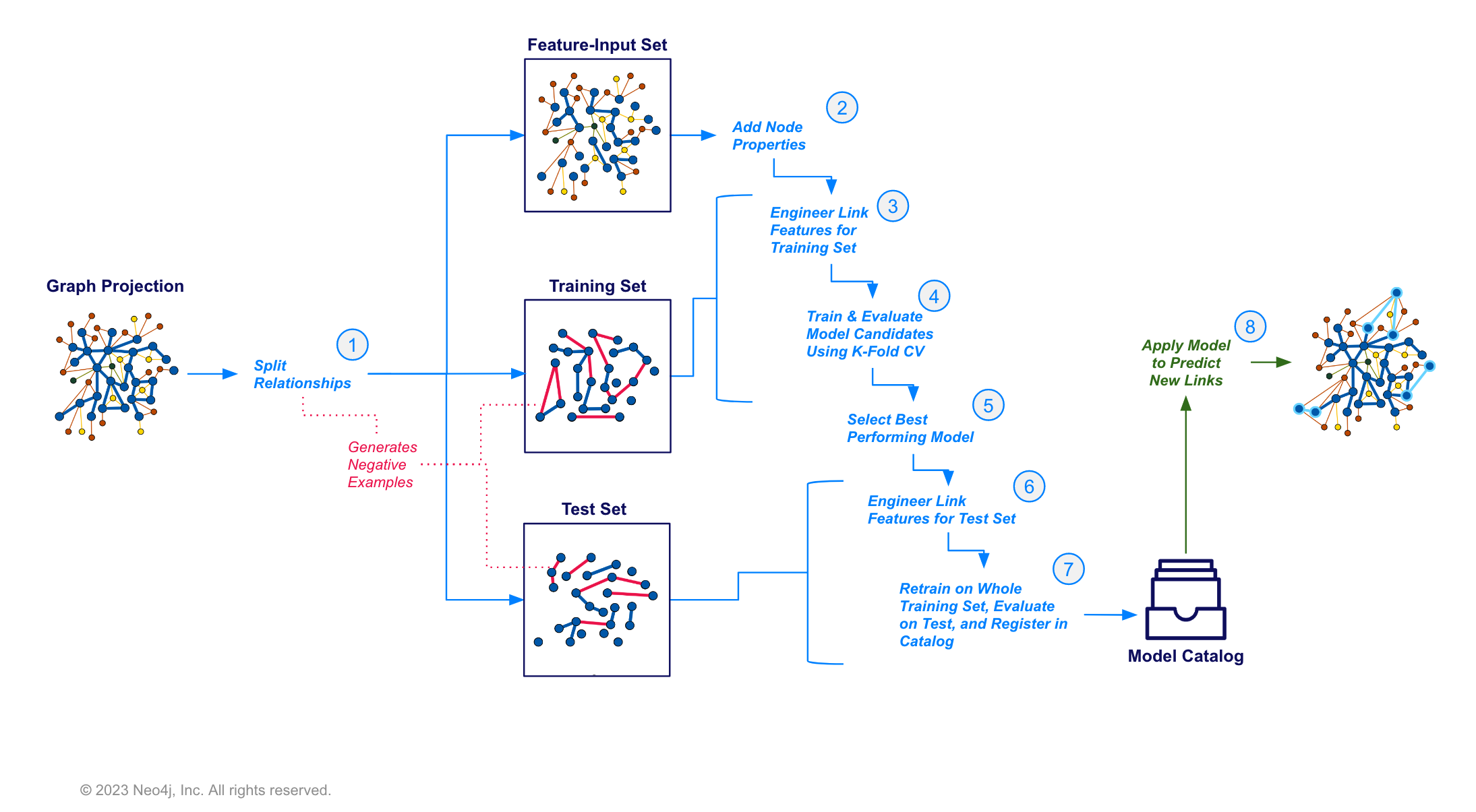
Node Classification Pipelines: Supervised binary and multi-class classification for nodes
Link Prediction Pipelines: Supervised prediction for whether a relationship or "link" should exist between pairs of nodes
These pipelines have a train procedure that, once run, produces a trained model object. These trained model objects, in turn, have a predict procedure that can be used to produce predictions on the data.
Node Classification Patterns in GDS
Shorted Path with Neo4j
We can either non-weighted or weighted shortestpath with neo4j. non-weighted in built in neo4j where for weighted we have to create a projections in noe4j.
Challenge: Dijkstra’s Source-Target Shortest Path
CALL gds.graph.project(
  'routes',
  'Airport',
  'HAS_ROUTE',
  {relationshipProperties:'distance'}
);
Find the Source-Target Shortest Path
MATCH (source:Airport {iata: "BNA"}),
      (target:Airport {iata:"HKT"})

CALL gds.shortestPath.dijkstra.stream(
  'routes',
  {
    sourceNode:source,
    targetNode:target,
    relationshipWeightProperty:'distance'
  }
) YIELD totalCost
RETURN totalCost;
Get K Multiple shorted Paths with yen’s algorithm
MATCH (source:Airport {iata: "CDG"}),
      (target:Airport {iata:"LIS"})

CALL gds.shortestPath.yens.stream(
  'routes',
  {
    sourceNode:source,
    targetNode:target,
    relationshipWeightProperty:'distance',
    k:3 // (1)
  })
YIELD index, nodeIds, totalCost // (2)
RETURN index, [nodeId in nodeIds | gds.util.asNode(nodeId).descr] AS airports, totalCost